Implementing regular expressions

Introduction

The first thing we do when we try to understand some program text is to divide it. For example, “12 + 34” can be divided into “12”, “+”, and “34”. If we want to include spaces, we can divide them as “12”, “ “, “+”, “ “, and “34”. Or if we are crazy, we can divide them as “12 +” and “34”.

The program texts are represented as strings. Before dividing a string, we need to decide on the rules for dividing. One set of rules can be we only care about numbers and the “+” sign. In that case, the valid substrings are “12”, “+”, and “34”.

These rules can be expressed as string patterns. Our problem can thus be phrased as dividing a string into substrings based on a set of patterns.

The substrings we divide a text into are called tokens. This process of dividing a string is called tokenization. We are going to implement a tokenizer in this article.

We will first look at the ways string patterns can be represented. Once we have these pattern representations, we are going to look at ways string patterns can be implemented. After we have discussed these implementations, we will put them together to implement a tokenizer.

This article assumes that you are comfortable with basic data structures and algorithms. We will use arrays, strings, hash tables, directed graphs, and recursion to develop the concepts in this article.

Representing string patterns

So how do we describe string patterns? One widely used notation is called regular expression. To understand regular expressions though, we need to define some new concepts.

The most basic thing we are dealing with is a string. A string can be empty or non-empty. An empty string is denoted by either "" or \(\epsilon\).

A set of strings is called a language.

For example, \(X = \{a, b, c\}\) is a language of three single character strings "a", "b", and "c". The language \(Y = \{abc, def\}\) has two strings "abc" and "def". And the language \(Z = \{xy\thinspace|\thinspace x \in \{a, b, c\} \thinspace and \thinspace y \in \{d, e, f\}\}\) is the same as \(W = \{ad, ae, af, bd, be, bf, cd, ce, cf\}\).

Languages are usually denoted by capital letters like A, B, X, and Y.

We combine languages using language operators. There are three language operators, union, concatenation, and kleene star, and we define them as follows.

The next operator is less intuitive than union and concatentation. The idea is to concatenate the strings from a single language. The number of concatenations can be zero, in which it case it is an empty string, upto any number of times.

Regular expressions

We now have all the tools we need to define regular expressions. Let’s start with an example. Suppose we want to represent all strings that consists of characters “a”, “b”, “c”, “1”, “2”, and “3”, such that they begin with “a”, “b”, and “c”.

What we just saw was an example of constructing a regular expression. Regular expressions are a way to combine language operators to represent string patterns.

The regular expression of the above pattern would be “(a|b|c)(a|b|c|1|2|3)*”.

Since regular expressions denote a set of strings, regular expressions describe a language.

Finite Automata

Finite automata is another mechanism to describe languages. Starting from directed graphs, we we will develop the concept of finite automata.

Transition tables and transition graphs

Suppose we have a directed graph where each vertex and edge is labeled. Here is an example.

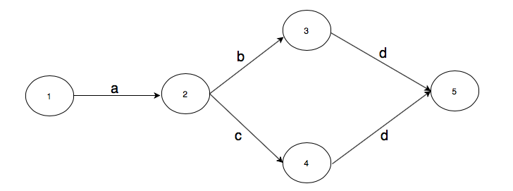
The adjacency list representation of the above graph is this.

{
  1: {"a": 2},
  2: {"b": 3, "c": 4},
  3: {"d": 5},
  4: {"d": 5}
}

In compiler terminology, vertices are called states, adjacency lists are called transition tables, and graphs themselves are called transition graphs. The edges of transition graphs are labeled by transition labels. The states in the above transition graph are 1, 2, 3, 4, and 5.

Transition graphs with initial and final states

Suppose we are in state 1 in the above graph. How can we reach state 5? We can reach it by either following the path

or

One path is labeled “abd” and the other path “acd”. We are beginning to see how transition graphs can define languages. Let’s designate one state as an initial state and one state as an accepting state. We represent the initial state in a transition graph by an arrow pointing from nowhere to that state. We represent an accepting state by using concentric circles for that state. In the above transition graph, if we designate 1 as an initial state and 5 as a final state, it would look like this.

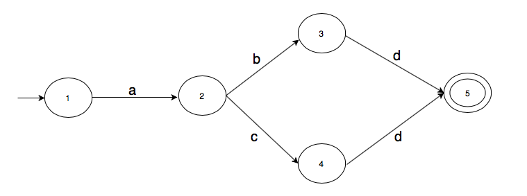
For this transition graph, we can say that strings “abc” and “abd” take it to the accepting state.

Let’s construct another transition graph, this time with multiple accepting states.

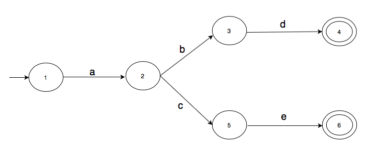
For this graph, strings “abd” and “ace” take the graph to an accepting state.

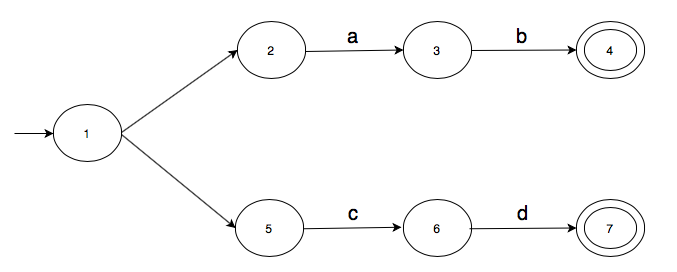
Transition graphs with empty string transitions

Going back to processing “ab”, we are in {1, 2, 5} and the next input character is “a”. There are no transitions labeled “a” out of states 1 and 5 but there is one from 2 to 3 with that label. So the next state is {3}.

Once we are in {3}, the next input character is “b” so we move to {4}. For “ab”, the transitions look like this.

compute_closure(S):
  closure_set = {S}

  if S has transitions out of it with label "":
    for each state T such that edge S-T has label "":
      closure_set = union(closure_set, compute_closure(T))

  return closure_set

At first, we initialise \(closure(1)\) to itself.

Thus,

Putting it all together, we can write the complete computation like this.

Finite automata

We now have all the pieces we need to define finite automata.

Let’s look at one of the earlier examples but as a finite automaton.

In this case:

1. \(Q = \{1, 2, 3, 4, 5, 6, 7, 8\}\)

2. \(q_0 = 1\)

3. \(F = \{4, 7\}\)

4. \(\Sigma = \{a, b, c, d\}\)

5. \(\delta.\) is represented by the following transition table.

{
  1: {"": {2, 5}},
  2: {"a": {3}, "": {8}},
  3: {"b": {4}},
  4: {},
  5: {"c": {6}},
  6: {"d": {7}},
  7: {},
  8: {}
}

Every finite automaton defines a language.

The language defined by the above automaton is {“ab”, “cd”}.

Implementing regular expressions using finite automata.

Both finite automata and regular expressions define languages. More importantly, every regular expression has an equivalent finite automaton. We won’t give a proof of this statement in this article.

Because regular expressions and finite automata are equivalent, we can implement regular expressions using finite automata.

In what follows, we will represent an arbitrary finite automata like this.

We defined regular expressions inductively. So we define the translation from regular expression to finite automaton for each basis and inductive case.

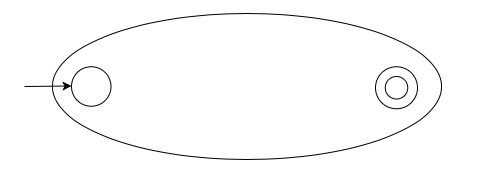
Basis case 1: Finite automata for regular expression “”

For regular expression “”, the equivalent finite automata is this.

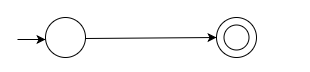
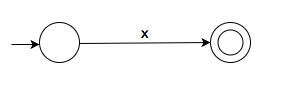
Basis case 2: Finite automata for a single character regular expression

For a single character regular expression like “x”, the equivalent finite automata is this.

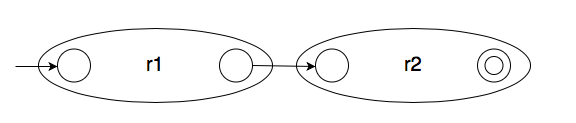
Inductive case 1: Union of two regular expressions

If we have two regular expressions r1 and r2, then their union r1|r2 has the following finite automaton. 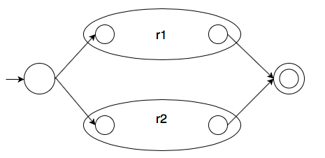That is, we do the following:

Inductive case 2: Concatenation of two regular expressions

If we have two regular expressions r1 and r2, then their concatenation, r1r2, has the following equivalent finite automata.

Inductive case 3: Kleene star of a regular expression

If we have a regular expression r1, then its kleene star, r1*, has the following equivalent finite automaton. 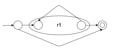That is, we do the following:

1. We create a new initial state and add an \(\epsilon\)-transition from that new initial state to the operand automaton's initial state.
2. We create a new accepting state and add an \(\epsilon\)-transition from the operand automaton's accepting state to the new accepting state.
3. We add an \(\epsilon\)-transition from the operand's accepting state to the operand's initial state.
4. We add an \(\epsilon\)-transition from the new initial state to the new accepting state.

Algorithm to implement regular expressions

The above inductive method can be translated into a recursive algorithm. Here is the pseudocode.

compile_regex_to_automaton(r):
  if (r is an empty string):
    return empty string finite automaton
  elif (r is a single character string):
    return single character finite automaton
  else:
    first_operand = get_first_operand(r)
    first_operand_automaton = compile_regex_to_automaton(first_operand)
  
    operator = get_operator(r)
    if operator is kleene star:
      # There is no second operand for kleene star.
      combined_automaton = apply_kleene_star(first_operand)
    else:
      second_operand = get_second_operand(r)
      second_operand_automaton = compile_regex_to_automaton(second_operand)
    
      if operator is union:
        combined_automaton = combine_using_union(first_operand_automaton, second_operand_automaton)
      else:
        combined_automaton = combine_using_concatenation(first_operand_automaton, second_operand_automaton)
    return combined_automaton
  }

Let’s run the above algorithm on regular expression is “(a|b)(c|d)*”. It will look like this.

compile_regex_to_automaton("(a|b)(c|d)*")
  compile_regex_to_automaton("(a|b)")
    first_operand_automaton = compile_regex_to_automaton("a")
    second_operand_automaton = compile_regex_to_automaton("b")
    automaton_for_a_b = combine_usion_union(first_automaton, second_automaton)
  compile_regex_to_automaton("(c|d)*")
    compile_regex_to_automaton("c|d")
      first_automaton = compile_regex_to_automaton("c")
      second_automaton = compile_regex_to_automaton("d")
      automaton_for_c_d = combine_using_union(first_automaton, second_automaton)
    automaton_for_c_d* = apply_kleene_star(automaton_for_c_d)
combine_using_concatenation(automaton_for_a_b, automaton_for_c_d*)

Tokenization

Using regular expressions and their finite automata implementations, we can implement a tokenizer. Given a set of regular expressions, a tokenizer divides a string into substrings.

Let’s look at an example. Suppose we have regular expressions for positive integers and arithemetic operators “+” and “*”. Given a string like “12*131+8”, we can use our regular expressions to divide it into substrings “12”, “*”, “131”, “+”, and “8”. The way we do that is we start from the left and bite off prefixes that match a regular expression. And we keep doing it until the string is empty.

So for “12*131+8”, we see that “12” will match the regular expression for positive integer. We bite that off and the remaining string is “*131+8”. Now, “*” will match the prefix so the remaining string is “131+8”. The number regex will match “131” and the remaining string will be “+8”. The regular expression for “+” will match the prefix and the remaining string will be “8”. Finally, the number regex will match “8” and all of the string will be exhausted.

Here’s a problem. What if multiple regular expressions match some prefix of the remaining string. For example, if the string is “==8” and we have regular expressions for both “=” and “==”, should we match the prefix “=” or “==”? In conflicts like these, we should always match the longest prefix possible. This policy is called the maximal munch policy.

The divided substrings are not returned as above but are used to construct objects called Tokens. Tokens represent the divided substrings and contain two pieces of information.

1. The regular expression used to match that substring. It is called the token type.
2. The substring matched for this token. It is called the lexeme.

We will represent a token as “<Tokentype, Lexeme>”. For example, the tokens for “12*131+8” are going to be “<positive_integer, 12>”, “<*, *>”, “<positive_integer, 131>”, “<+, +>”, and “<positive_integer, 8>”.

Thus the output of a tokenizer is an array of tokens. These tokens are inputs to later phases of the compiler.

Conclusion

Here’s a Go implementation of a tokenizer.