Constructing basic blocks

In this article, we cover concepts from the second lesson of the advanced compilers course from Cornell. However, the specific algorithms discussed in this article are different from the ones discussed in the course.

Introduction

To execute a program written in a high level-language, we first need to translate it into a processor-specific machine language program. One way to do this is to first translate the program text into a data structure. We can then use that data structure to generate a machine language program. These intermediary data structures are called intermediate representations.

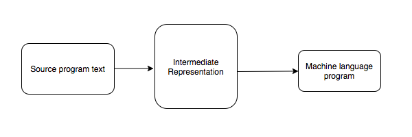
These intermediate representation languages are closer to assembly languages than the source languages. They have more primitive operators and more primitive control flow facilities. The intermediate representations are effectively abstracted assembly languages that do not have various architecture quirks.

A benefit of this design is that we can translate multiple source languages into an intermediate representation. That intermediate representation can then generate different processor-specific programs. It is easier to write new languages for existing architectures and for an existing compiler to target new architectures.

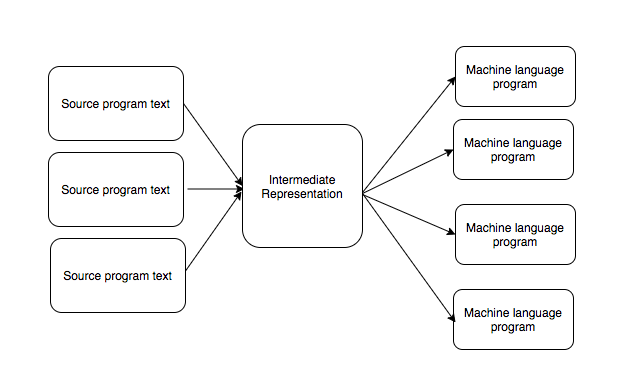
Another benefit of this design is that the analyses and transformations done on intermediate representations remain intact when we generate machine code from that intermediate representation. It’s a consequence of intermediate representations being a good model of the processor specific languages.

Some examples of intermediate representations are Llvm IR and Java bytecode.

In this article, we will study a method of grouping instructions written in an intermediate language. These instruction groups are called basic blocks. We will start by describing the relevant parts of the IR language that we will be using. After that, we will represent our program using a data structure called the control flow graph. And finally, we will use the control flow graph representation to construct basic blocks.

Relevant intermediate representation (IR) background

We will be using Bril intermediate representation which came out of the Capra group at Cornell. We will restrict ourselves to the following features of Bril.

1. Bril programs have a textual representation and a json representation. These representations are interchangeble.
2. The Bril programs under consideration will have only one function named main.
3. Labels mark specific points in a program. They are used to refer to instructions by other instructions of a program.
4. An instruction can be either a label or an operation.
5. There are two control flow instructions: jmp and br.
6. The jmp is an unconditional jump that takes one argument, the label to jump to.
7. The br is a conditional jump that takes three arguments. It takes a variable of type bool and two labels. The program jumps to the first label if the variable is true and the second label otherwise.

More details about bril can be found in the documentation.

Here are some examples. Below is a simple program that prints a constant.

@main {
  v: int = const 4;
  print v;
}

Its json representation is this.

{
  "functions": [
    {
      "name": "main",
      "instrs": [
        {"dest": "v", "type": "int", "op": "const", "value": 4},
        {"op": "print", "args": ["v"]}
      ]
    }
  ]
}

Here’s a program that uses the jmp instruction to do an unconditional jump to a label.

@main {
  v: int = const 4;
  jmp .somewhere;
  v: int = const 2;
.somewhere:
  print v;
}

Its json representation is this.

{
  "functions": [
    {
      "name": "main",
      "instrs": [
        {"dest": "v", "type": "int", "op": "const", "value": 4},
        {"op": "jmp", "labels": ["somewhere"]},
        {"dest": "v", "type": "int", "op": "const", "value": 2},
        {"label": "somewhere"},
        {"op": "print", "args": ["v"]}
      ]
    }
  ]
}

And here’s a program that uses br to do a conditional jump.

@main {
  v: int = const 4;
  b: bool = const false;
  br b .there .here;
.here:
  v: int = const 2;
.there:
  print v;
}

Here, the value of b determines whether the jump is going to here or there. Since the value of b is hardcoded to false in this example, it will always jump to the .here label. The json representation looks like this.

{
  "functions": [
    {
      "name": "main",
      "instrs": [
        {"dest": "v", "type": "int", "op": "const", "value": 4},
        {"dest": "b", "type": "bool", "op": "const", "value": false},
        {"op": "br", "args": ["b"], "labels": ["there", "here"]},
        {"label": "here"},
        {"dest": "v", "type": "int", "op": "const", "value": 2},
        {"label": "there"},
        {"op": "print", "args": ["v"]}
      ]
    }
  ]
}

Control flow graph

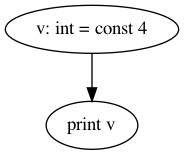
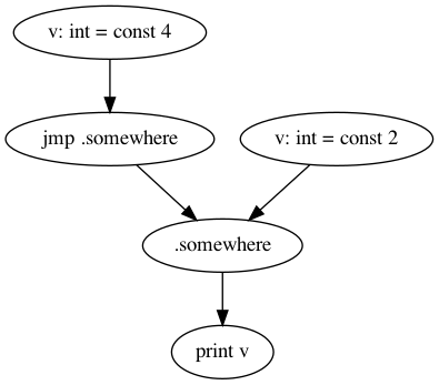
A control flow graph represents the flow of control of a function. Each instruction is a vertex in the graph and the vertices are connected according to the flow of control of instructions.

For example, for the program

@main {
  v: int = const 4;
  print v;
}

the control flow graph will looks like this.

For the program

@main {
  v: int = const 4;
  jmp .somewhere;
  v: int = const 2;
.somewhere:
  print v;
}

it will look like this.

To construct the control flow graph for a program, we need to compute the instructions that we can directly go to from each instruction. In our intermediate representation, the answers are as follows.

1. If the instruction is neither a jmp nor a br, the reachable instruction is the next instruction in the instruction array.
2. If the instruction is a jmp, the next instruction is the instruction identified by the label of the jump.
3. If the instruction is a br, there are two instructions reachable from that instruction, identified by the labels of the instruction.

Points 2. and 3. refer to labels. To construct the control flow graph, we first need to associate labels with their corresponding instructions. Let’s clarify this with an example. Here’s the json representation of our jmp program.

{
  "functions": [
    {
      "name": "main",
      "instrs": [
        {"dest": "v", "type": "int", "op": "const", "value": 4},
        {"op": "jmp", "labels": ["somewhere"]},
        {"dest": "v", "type": "int", "op": "const", "value": 2},
        {"label": "somewhere"},
        {"op": "print", "args": ["v"]}
      ]
    }
  ]
}

In Bril, an instruction is a label if it has the label property. There is only one such instruction in this program, {"label": "somewhere"}, which is the second last instruction.

Before constructing the control flow graph, we need to map labels to indices of instructions in the instruction array. Here is a python implementation of this idea which takes the instrs list from the json representation as input.

def map_labels_to_instructions(instrs):
    label_to_instruction = {}
    for idx, instr in enumerate(self.instrs):
        if "label" in instr:  # is the instruction a label?
            label_to_instruction[instr["label"]] = idx

    return label_to_instruction

Let’s do an example run of the above program. For the br program reproduced below,

{
  "functions": [
    {
      "name": "main",
      "instrs": [
        {"dest": "v", "type": "int", "op": "const", "value": 4},
        {"dest": "b", "type": "bool", "op": "const", "value": false},
        {"op": "br", "args": ["b"], "labels": ["there", "here"]},
        {"label": "here"},
        {"dest": "v", "type": "int", "op": "const", "value": 2},
        {"label": "there"},
        {"op": "print", "args": ["v"]}
      ]
    }
  ]
}

the output would be the following dictionary.

{
    "here": 3,
    "there": 5
}

We are ready to construct the control flow graph of a program. We will represent this graph using adjacency list representation. For each instruction, we need to figure out the instructions it can go to.

def construct_graph(instrs):
    label_to_instruction = map_labels_to_instructions(instrs)
    graph = collections.defaultdict(set)  # Adjacency list representation of program

    for idx, instr in enumerate(self.instrs):
        if "op" in instr and instr["op"] in {"jmp", "br"}:
            # It is a jmp or a br. Find destination instruction indexes corresponding to labels and connect
            # them to this instruction index.
            for label in instr["labels"]:
                dest_instr_idx = label_to_instruction[label]
                graph[idx].add(dest_instr_idx)
        elif idx < len(self.instrs) - 1:
            # Its not the last instruction. Connect it to the subsequent instruction.
            graph[idx].add(idx + 1)
    return graph

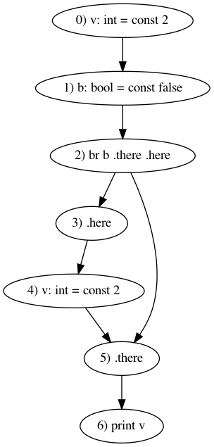
This program is identifying each instruction with its array index. For our above br program, it will construct this dictionary.

{
    0: {1},
    1: {2},
    2: {3, 5},
    3: {4},
    4: {5},
    5: {6},
}

Pictorially, it will look like this. We have labelled vertices here with instruction numbers and their corresponding instructions.

Basic blocks

We now have all the concepts we need to discuss basic blocks. A basic block is a sequence of instructions such that:

1. Executing its first instruction guarantees that all instructions within that block will execute.
2. We can enter a block via the first instruction only. There is no other entry point for a basic block.

Let’s construct basic blocks for the following program.

@main {
  v: int = const 4;
  b: bool = const false;
  br b .there .here;
.here:
  v: int = const 2;
.there:
  print v;
  jmp .here;
}

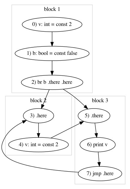
Starting from the first instruction, we can see that if v: int = const 4; executes, then b: bool = const false; will definitely execute. And if b: bool = const false; executes, then br b .there .here will definitely execute.

It could happen that .here executes after br b .there .here. But .here will also execute after the last instruction jmp .here. According to the second point of our definition, we can only enter a basic block via its first instruction. Thus, we must finish our current block at br b .there .here and start a new one at .here.

If .here executes, then v: int = const 2 will definitely execute. And while its true that the execution of v: inst = const 2 implies the execution of .there, it is also true that .there could follow br b .there .here. Thus, v: int = const 2 should end the current block and .there should start a new block.

Similarly, the block starting from .there ends at jmp .here.

The below figure shows the control flow graph of the above program with the basic blocks marked by gray boxes.

Let’s convert our above intuition into an algorithm and its implementation. Since we are modeling our list of instructions as graphs, we should translate the requirements of basic blocks into graphical terms. We can re-express the two criteria like this.

1. Each vertex in a block except the last one has one outgoing edge. The last vertex can have either no outgoing edge or multiple outgoing edges.
2. Each vertex in a block except the first has one incoming edge. The first vertex can have either no incoming edge or multiple incoming edges.

We can check the first requirement for each vertex by doing a depth-first search on the graph. To check the second requirement, we need to compute the parent vertices for each vertex. We can determine the parent vertices for each vertex by doing a breadth-first search on our control flow graph. The python implementation is as follows.

def construct_child_parent_relationship(graph):
    child_to_parent = collections.defaultdict(set)  # Each vertex can have multiple parents.
    queue = collections.deque()
    unvisited = {idx for idx in range(1, len(self.instrs))}
    
    queue.append(0)  # Start from the first vertex.
    while queue:
        # Main BFS loop.
        current_vertex = queue.popleft()
        for next_vertex in self.graph[current_vertex]:
            # Whether or not we have seen next_vertex before, add current_vertex as its parent.
            child_to_parent[next_vertex].add(current_vertex)
            if next_vertex in unvisited:
                unvisited.remove(next_vertex)
                queue.append(next_vertex)

        if not queue and unvisited:
            # If the queue is empty but there are still some unvisited vertices, pop a random
            # unvisited vertex into the queue.
            queue.append(unvisited.pop())

    return child_to_parent

We are now ready to group vertices into basic blocks. We start with the first instruction and keep constructing new basic blocks till we have exhausted all the instructions. We do this using a depth-first search. Because we have several state variables related to basic blocks, it would be easier to do it using an iterative depth-first search. Here is an implementation of our two requirements. Because the code is relatively more involved, we run it on one of our example programs right after the code.

def construct_basic_blocks(instrs):
    child_to_parent = self.construct_child_parent_relationship()
    stack = [0]
    basic_blocks = []
    current_block = []
    unvisited = {idx for idx in range(1, len(self.instrs))}
    while stack:
        current_vertex = stack.pop()
        if not current_block or len(child_to_parent[current_vertex]) == 1:
            current_block.append(current_vertex)
        else:
            basic_blocks.append(current_block)
            current_block = [current_vertex]

        if len(self.graph[current_vertex]) != 1:
            # If the current vertex has either zero children or more than one children, it must terminate
            # the current block and we must start a new block. Multiple edges cannot come out from within
            # a block.
            basic_blocks.append(current_block)
            current_block = []

        unvisited_children = {vertex for vertex in self.graph[current_vertex] if vertex in unvisited}
        if not unvisited_children:
            # No child for the current vertex. End current block and start a new block.
            basic_blocks.append(current_block)
            current_block = []
        else:
            # Continue dfs on unseen children.
            for next_vertex in unvisited_children:
                unvisited.remove(next_vertex)
                stack.append(next_vertex)
            
        if not stack and unvisited:
            # If the stack is empty but there are some unprocessed vertices, add them to the stack.
            stack.append(unvisited.pop())

    basic_blocks = [current_block for current_block in basic_blocks if current_block]
    basic_blocks.sort()
    return basic_blocks

Let’s run this code on the below program. To make it easy to read, we converted the instrs array into an object with indices. It will help in relating instructions to their indices.

{
  "functions": [
    {
      "name": "main",
      "instrs": {
        0: {"dest": "v", "type": "int", "op": "const", "value": 4},
        1: {"dest": "b", "type": "bool", "op": "const", "value": false},
        2: {"op": "br", "args": ["b"], "labels": ["there", "here"]},
        3: {"label": "here"},
        4: {"dest": "v", "type": "int", "op": "const", "value": 2},
        5: {"label": "there"},
        6: {"args": ["v"], "op": "print"},
        7: {"labels": ["here"], "op": "jmp"}
      },
    }
  ]
}

The control flow graph and the child to parent relationships for the above program looks like this.

control_flow_graph = {0: {1}, 1: {2}, 2: {3, 5}, 3: {4}, 4: {5}, 5: {6}, 6: {7}, 7: {3}}
child_parent_dict = {1: {0}, 2: {1}, 3: {2, 7}, 5: {2, 4}, 4: {3}, 6: {5}, 7: {6}}

We are now ready to simulate our construct_basic_blocks function. Here are the four variables that we will track along with their initial values.

basic_blocks = []
current_block = []
stack = [0]
unvisited = {1, 2, 3, 4, 5, 6, 7}

We enter the while loop of line 7 for the first time. Because the current_block is empty, the if block of line 9 will execute. Since there is only one child of 1, the if block of line 15 won’t execute. And since there is an unvisited child of vertex 0, the else block of line 27 will execute. The if block of line 33 will not execute. The situation looks like this now.

basic_blocks = []
current_block = [0]
stack = [1]
unvisited = {2, 3, 4, 5, 6, 7}

Entering the while loop again, the if block on line 9 will execute because 1 has only one parent. And since 1 has one unvisited child, the if block of line 15 won’t execute and the else block of line 27 will execute. The if block of line 33 will again be skipped. After second iteration, the variables look like this.

basic_blocks = []
current_block = [0, 1]
stack = [2]
unvisited = {3, 4, 5, 6, 7}

The next iteration of the while loop will be different. The current vertex 2 has just one parent so it will be added to the current block. But vertex 2 has two children so we will end the current block in the if block of line 15 and start a new block. Since the children of 2 are in unvisited, we add them to the stack in the else block of line 27.

basic_blocks = [[0, 1, 2]]
current_block = []
stack = [3, 5]
unvisited = {4, 6, 7}

Now 5 will be our current vertex. Because 5 has two parents, 2 and 4, the current block ends and a new block is initalised with 5 in the else block of line 11. Since 5 has an unvisited child, the else block of line 27 will execute. The if block of line 33 will not execute.

basic_blocks = [[0, 1, 2]]
current_block = [5]
stack = [3, 6]
unvisited = {4, 7}

Now the current vertex is 6 which has one parent and one unvisited child so the state variables look like this.

basic_blocks = [[0, 1, 2]]
current_block = [5, 6]
stack = [3, 7]
unvisited = {4}

The current vertex is 7 which has one parent but has no unvisited child. We therefore end the current block and start a new one. The variables look like this now.

basic_blocks = [[0, 1, 2], [5, 6, 7]]
current_block = []
stack = [3]
unvisited = {4}

The current block is empty so we initialise a new block in the if of line 9 with 3. 3 has one unvisited children which we add to the stack.

basic_blocks = [[0, 1, 2], [5, 6, 7]]
current_block = [3]
stack = [4]
unvisited = {}

Now, the vertex 4 has just one parent and no unvisited child. The stack would be empty now and there are no unvisited vertices left. 4 will be added to the current block in the if block of line 9. There are no unvisited vertices left so the current block will be appended to the list of basic blocks in the if block of line 23. There will no more iterations of the while loop.

basic_blocks = [[0, 1, 2], [5, 6, 7], [3, 4]]
current_block = []
stack = []
unvisited = {}

After the loop, we remove empty blocks and sort basic blocks. Sorting helps in recombining basic blocks to form a complete list of instructions. The final result will look like this.

basic_blocks = [[0, 1, 2], [3, 4], [5, 6, 7]]

The basic blocks we computed using this function match the ones we computed intutively using graph above.

Conclusion

Breaking a list of instructions into basic blocks is the first step towards compiler optimizations. In a next article, we will discuss optimizations that we can do within a basic block.